Graph of Uniform Linear Motion

In this lecture, we will consider graphing uniform linear motion. Some people are intimidated when they hear the word “graph,” but it is not difficult at all.
Using graphs, you can visualize motion, solve problems that would be difficult to calculate directly, and more!

1. x-t Graph

The three main components of uniform linear motion are speed, distance, and time, but since we cannot graph all three together, we will pick up two of the three and graph them.

So, first of all, here is a graph showing the relationship between x (Distance) and t (Time).

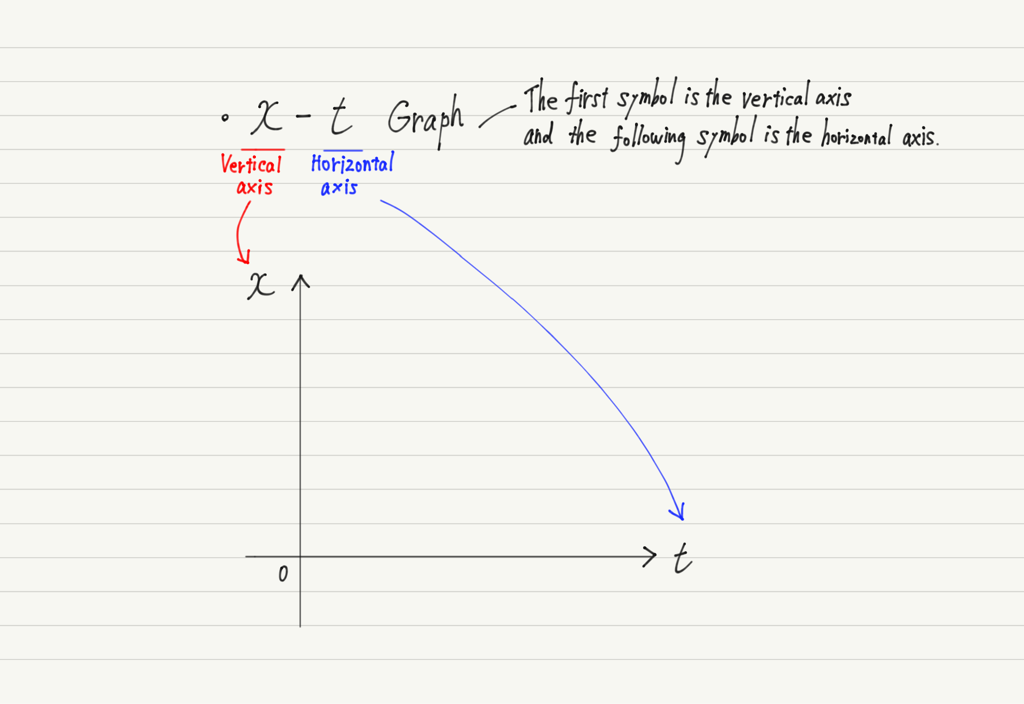
What will be the shape of the graph?

For example, if we consider an object moving at a constant speed of 10 m/s, this means that it will move 10 m per second, so it will move 20 m in 2 seconds, 30 m in 3 seconds, and 100 m in 10 seconds.

Thus, as time doubles or triples, the distance traveled also doubles or triples.

That demonstrates proportionality!

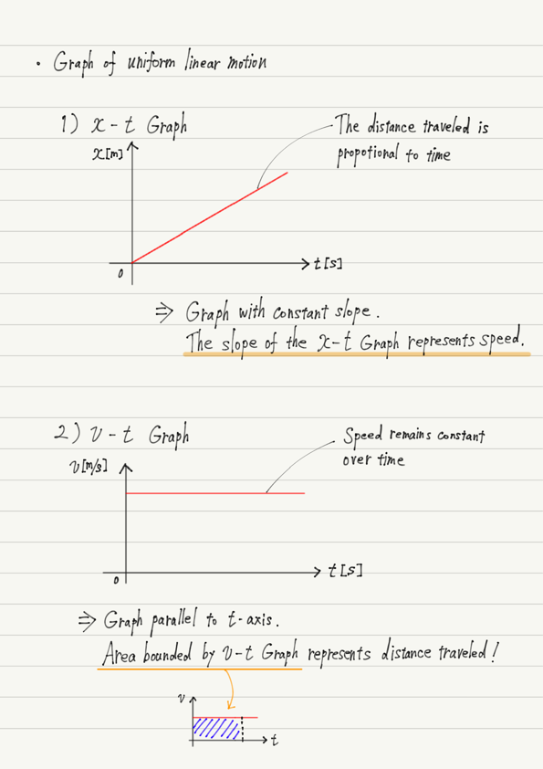
In uniform linear motion, the distance traveled increases in proportion to the time taken, so the x-t graph becomes a graph of a straight line.

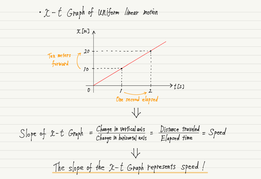
It is important to note that the slope of the x-t graph represents speed. The greater the slope of the graph, the faster the motion.

2. v-t Graph

Next, we have a graph showing the relationship between v (Speed) and t (Time). This graph shows “How does the velocity change with time?”

Since this is a uniform linear motion, the speed does not change no matter how much time passes.

Consider an object moving at a constant speed of 10 m/s, and the graph is as follows.

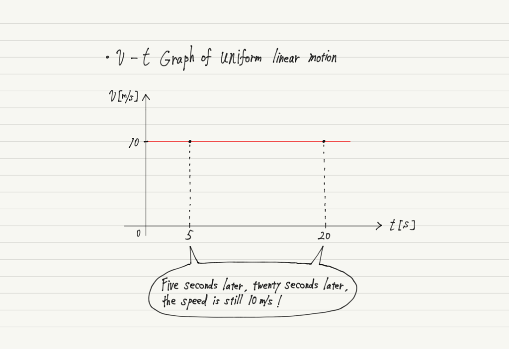
It’s a very simple graph.

Now, let’s separate this graph at an appropriate time (e.g., t=20 s).

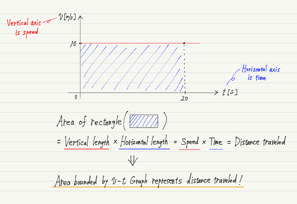
Thus, the area enclosed by the v-t graph and the t-axis represents the distance traveled!

Keep this in mind, as it will be used later. That’s all for this lecture!

Summary of this lecture

Next lecture preview

Next time I would like to stop and review some of the terms.

Related articles

Speed and Velocity